Assessing variable importance in survival analysis using machine learning

library(survML)
#> Loading required package: SuperLearner
#> Loading required package: nnls
#> Loading required package: gam
#> Loading required package: splines
#> Loading required package: foreach
#> Loaded gam 1.22-4
#> Super Learner
#> Version: 2.0-29
#> Package created on 2024-02-06
library(survival)
library(dplyr)
#> 
#> Attaching package: 'dplyr'
#> The following objects are masked from 'package:stats':
#> 
#>     filter, lag
#> The following objects are masked from 'package:base':
#> 
#>     intersect, setdiff, setequal, union
library(ggplot2)
set.seed(72924)

Introduction

The survML package includes functions that can be used to estimate model-free, algorithm-agnostic variable importance when the outcome of interest is subject to right censoring. Specifically, this functionality is aimed at estimating intrinsic variable importance, which is the population-level predictiveness potential of a feature or group of features.

Suppose we have access to a vector $X$ of features, which we wish to use to make a prediction involving $T$, a time-to-event outcome. We use $C$ to denote the right censoring variable. The observed data are given by $(X, Y, \Delta)$, where $\Delta := I(T \leq C)$ and $Y := \text{min}(T, C)$. For an index set $s$, we use $X_s$ to denote the elements of $X$ with index in $s$ and $X_{-s}$ its complement. For a given prediction task (say, estimating the probability that $T$ is smaller than some landmark time $\tau$) and prediction function $f$, we require a measure of predictiveness. We let $V(f, P_0)$ denote the predictiveness of $f$ under sampling from distribution $P_0$. We define $f_{0,s}$ as the oracle prediction function excluding features with index in $s$; this is the best possible prediction function, according to $V$, that uses only $X_{-s}$.

For intrinsic variable importance, we consider nested index sets $r \subset s$ and define the importance of $X_{s \setminus r}$ relative to $X_s$ as $V(f_{0,r}, P_0) - V(f_{0,s}, P_0)$; this is the difference in maximum achievable predictiveness when only $r$ is excluded compared to when $s$ is excluded. We refer to this parameter as a variable importance measure (VIM).

Due to right censoring, the VIM estimation procedure requires estimates of the conditional survival functions of $T$ and $C$ given $X$, which we define pointwise as $S_0(t \mid x) := P_0(T > t \mid X = x)$ and $G_0(t \mid x) := P_0(C > t \mid X = x)$, respectively. These functions must be estimated over the interval $(0, \tau]$ and may be obtained from any conditional survival estimation algorithm. This may be as simple as a Cox proportional hazards model (Cox, 1972) or parametric survival regression model, or as complex as a stacked regression procedure such as survival Super Learner (Westling et al., 2023) or global survival stacking (Wolock et al., 2024).

We also require estimates of the oracle prediction functions $f_{0,r}$ and $f_{0,s}$, whose exact form depends on the chosen predictiveness measure. For several commonly used measures, the oracle prediction functions can be written in terms of $S_0(\cdot \mid x)$. The form of the oracle prediction function for the measures included in survML is given in the Appendix.

Example: Predicting recurrence-free survival time in cancer patients

As an example, we consider estimating variable importance for predicting recurrence-free survival using the gbsg dataset in the survival package. The Kaplan-Meier estimate of the survival curve for this dataset is shown below.

data(cancer)
km_fit <- survfit(Surv(rfstime, status) ~ 1, data = gbsg)
plot(km_fit, xlab = "Time (days)", ylab = "Recurrence-free survival probability")

We will consider time-varying AUC importance using landmark times of 500, 1000, 1500 and 2000 days. The first step is to prepare the data. We use dummy coding for factors. This means that to assess the importance of tumor grade, for example, which has three levels, we create two dummy variables called tumgrad2 and tumgrad3 and consider them as a single feature group. We also consider the feature groups defined by tumor-level features and patient-level features.

### variables of interest
# rfstime - recurrence-free survival
# status - censoring indicator
# hormon - hormonal therapy treatment indicator
# age - in years
# meno - 1 = premenopause, 2 = post
# size - tumor size in mm
# grade - factor 1,2,3
# nodes - number of positive nodes
# pgr - progesterone receptor in fmol
# er - estrogen receptor in fmol

# create dummy variables and clean data
gbsg$tumgrad2 <- ifelse(gbsg$grade == 2, 1, 0)
gbsg$tumgrad3 <- ifelse(gbsg$grade == 3, 1, 0)
gbsg <- gbsg %>% na.omit() %>% select(-c(pid, grade))

time <- gbsg$rfstime
event <- gbsg$status
X <- gbsg %>% select(-c(rfstime, status)) # remove outcome 

# find column indices of features/feature groups
X_names <- names(X)
age_index <- paste0(which(X_names == "age"))
meno_index <- paste0(which(X_names == "meno"))
size_index <- paste0(which(X_names == "size"))
nodes_index <- paste0(which(X_names == "nodes"))
pgr_index <- paste0(which(X_names == "pgr"))
er_index <- paste0(which(X_names == "er"))
hormon_index <- paste0(which(X_names == "hormon"))
grade_index <- paste0(which(X_names %in% c("tumgrad2", "tumgrad3")), collapse = ",")
tum_index <- paste0(which(X_names %in% c("size", "nodes", "pgr", "er", "tumgrad2", "tumgrad3")),
                    collapse = ",")
person_index <- paste0(which(X_names %in% c("age", "meno", "hormon")), collapse = ",")

feature_group_names <- c("age", "meno.", "size", "nodes",
                         "prog.", "estro.", "hormone", 
                         "grade")
feature_groups <- c(age_index, meno_index, size_index, nodes_index,
                    pgr_index, er_index, hormon_index, grade_index)

# consider joint importance of all tumor-level and person-level features
feature_group_names2 <- c("tumor", "person")
feature_groups2 <- c(tum_index, person_index)

Next, we write some functions to estimate all the relevant nuisance parameters.

# estimate conditional survival functions
generate_nuisance_predictions <- function(time, 
                                          event, 
                                          X, 
                                          X_holdout, 
                                          newtimes,
                                          approx_times,
                                          SL.library){
  
  surv_out <- survML::stackG(time = time,
                             event = event,
                             X = X,
                             newX = rbind(X_holdout, X),
                             newtimes = approx_times,
                             time_grid_approx = approx_times,
                             bin_size = 0.05,
                             time_basis = "continuous",
                             surv_form = "PI",
                             SL_control = list(SL.library = SL.library,
                                               V = 5))
  S_hat <- surv_out$S_T_preds[1:nrow(X_holdout),]
  G_hat <- surv_out$S_C_preds[1:nrow(X_holdout),]
  S_hat_train <- surv_out$S_T_preds[(nrow(X_holdout)+1):(nrow(X_holdout)+nrow(X)),]
  G_hat_train <- surv_out$S_C_preds[(nrow(X_holdout)+1):(nrow(X_holdout)+nrow(X)),]
  return(list(S_hat = S_hat,
              G_hat = G_hat,
              S_hat_train = S_hat_train,
              G_hat_train = G_hat_train))
}


generate_full_oracle_predictions <- function(time,
                                             event,
                                             X,
                                             X_holdout,
                                             nuisance_preds,
                                             landmark_times,
                                             approx_times){
  
  f0_hat <- nuisance_preds$S_preds[,which(approx_times %in% landmark_times),drop=FALSE]
  f0_hat_train <- nuisance_preds$S_preds_train[,which(approx_times %in% landmark_times),drop=FALSE]
  return(list(f0_hat = f0_hat,
              f0_hat_train = f0_hat_train))
  
}

generate_reduced_oracle_predictions <- function(time,
                                                event,
                                                X,
                                                X_holdout,
                                                nuisance_preds,
                                                landmark_times,
                                                approx_times,
                                                SL.library,
                                                indx){
  X_reduced_train <- X[,-indx,drop=FALSE]
  X_reduced_holdout <- X_holdout[,-indx,drop=FALSE]
  preds_j <- matrix(NA, nrow = nrow(X_reduced_holdout), ncol = length(landmark_times))
  preds_j_train <- matrix(NA, nrow = nrow(X_reduced_train), ncol = length(landmark_times))
  
  for (t in landmark_times){
    outcomes <- nuisance_preds$full_preds_train[,which(landmark_times == t)]
    long_dat <- data.frame(f_hat = outcomes, X_reduced_train)
    long_new_dat <- data.frame(X_reduced_holdout)
    long_new_dat_train <- data.frame(X_reduced_train)
    reduced_fit <- SuperLearner::SuperLearner(Y = long_dat$f_hat,
                                              X = long_dat[,2:ncol(long_dat),drop=FALSE],
                                              family = stats::gaussian(),
                                              SL.library = SL.library,
                                              method = "method.NNLS",
                                              verbose = FALSE)
    reduced_preds <- matrix(predict(reduced_fit, newdata = long_new_dat)$pred,
                            nrow = nrow(X_reduced_holdout),
                            ncol = 1)
    reduced_preds_train <- matrix(predict(reduced_fit, newdata = long_new_dat_train)$pred,
                                  nrow = nrow(X_reduced_train),
                                  ncol = 1)
    preds_j[,which(landmark_times == t)] <- reduced_preds
    preds_j_train[,which(landmark_times == t)] <- reduced_preds_train
  }
  
  return(list(f0_hat = preds_j,
              f0_hat_train = preds_j_train))
}

Estimating variable importance relative to all features

First, we consider the importance of each of the feature groups relative to the full feature vector. Here, the features of interest are subtracted from the full feature vector, with importance measured by the resulting loss in predictiveness.

Note that because censoring may be informed by covariates that are not part of the current reduced feature set, we estimate the residual oracle prediction function by regressing the full oracle predictions on the reduced feature set, rather than directly estimating the conditional survival function using the reduced feature set.

To reduce runtime, we use a very small Super Learner library. In actual analyses, it is generally a good idea to use a larger library of learners.

# super learner library for global survival stacking
SL.library <- c("SL.mean", "SL.glm")

# landmark times for AUC
landmark_times <- c(500, 1000, 1500, 2000)

# set up cross-fitting and sample-splitting folds
cf_fold_num <- 2
ss_fold_num <- 2*cf_fold_num
V <- ss_fold_num
folds <- sample(rep(seq_len(V), length = nrow(gbsg))) # 2V of them
ss_folds <- c(rep(1, V/2), rep(2, V/2))
ss_folds <- as.numeric(folds %in% which(ss_folds == 2))

# approximation time grid for integrals 
approx_times <- sort(unique(c(time[event == 1 & time <= max(landmark_times)], 
                              landmark_times)))

# generate nuisance estimates
nuisance_preds <- crossfit_surv_preds(time = time,
                                      event,
                                      X = X,
                                      newtimes = approx_times,
                                      folds = folds,
                                      pred_generator = generate_nuisance_predictions,
                                      SL.library = SL.library,
                                      approx_times = approx_times)

CV_S_preds <- nuisance_preds$S_preds
CV_S_preds_train <- nuisance_preds$S_preds_train
CV_G_preds <- nuisance_preds$G_preds

full_preds <- crossfit_oracle_preds(time = time,
                                    event = event,
                                    X = X,
                                    folds = folds,
                                    nuisance_preds = nuisance_preds,
                                    pred_generator = generate_full_oracle_predictions,
                                    landmark_times = landmark_times,
                                    approx_times = approx_times)

CV_full_preds <- full_preds$oracle_preds
CV_full_preds_train <- full_preds$oracle_preds_train

augmented_nuisance_preds <- nuisance_preds
augmented_nuisance_preds$full_preds_train <- CV_full_preds_train

# iterate over feature groups
for (i in 1:length(feature_group_names)){
  indx_char <- feature_groups[i]
  indx_name <- feature_group_names[i]
  indx <- as.numeric(strsplit(indx_char, split = ",")[[1]])
  
  reduced_preds <- crossfit_oracle_preds(time = time,
                                         event = event,
                                         X = X,
                                         folds = folds,
                                         nuisance_preds = augmented_nuisance_preds,
                                         pred_generator = generate_reduced_oracle_predictions,
                                         landmark_times = landmark_times,
                                         approx_times = approx_times,
                                         SL.library = SL.library,
                                         indx = indx)
  CV_reduced_preds <- reduced_preds$oracle_preds
  
  # estimate VIM - note the oracle for AUC is the conditional cdf, not survival function, 
  # so need to take 1 - S(tau | x)
  output <- vim_AUC(time = time,
                    event = event,
                    approx_times = approx_times,
                    landmark_times = landmark_times,
                    f_hat = lapply(CV_full_preds, function(x) 1-x),
                    fs_hat = lapply(CV_reduced_preds, function(x) 1-x),
                    S_hat = CV_S_preds,
                    G_hat = CV_G_preds,
                    folds = folds,
                    ss_folds = ss_folds,
                    sample_split = TRUE,
                    scale_est = TRUE)
  
  output$vim <- "AUC"
  output$indx <- rep(indx_char, nrow(output))
  output$indx_name <- rep(indx_name, nrow(output))
  if (!(i == 1)){
    pooled_output <- rbind(pooled_output, output)
  } else{
    pooled_output <- output
  }
}

# plot results
p_auc <- pooled_output %>%
   mutate(landmark_time = factor(landmark_time,
                                levels = c(500, 1000, 1500, 2000),
                                labels = c("500 days", "1000 days", "1500 days", "2000 days"))) %>%
  arrange(landmark_time, est) %>%
  mutate(Order = row_number()) %>%
  {ggplot(., aes(x = est, y = Order)) +
      geom_errorbarh(aes(xmin = cil, xmax = ciu)) +
      geom_point() +
      theme_bw() +
      xlab("Estimated importance") +
      ylab("Feature group") +
      xlim(c(0,0.3)) +
      scale_y_continuous(
        breaks = .$Order,
        labels = .$indx_name,
      ) + 
      facet_wrap(~landmark_time, dir = "v", strip.position = "right", scales = "free_y", ncol = 1) + 
      ggtitle("AUC variable importance relative to full feature vector")+
      theme(strip.background = element_blank(),
            strip.placement = "outside")
  }
p_auc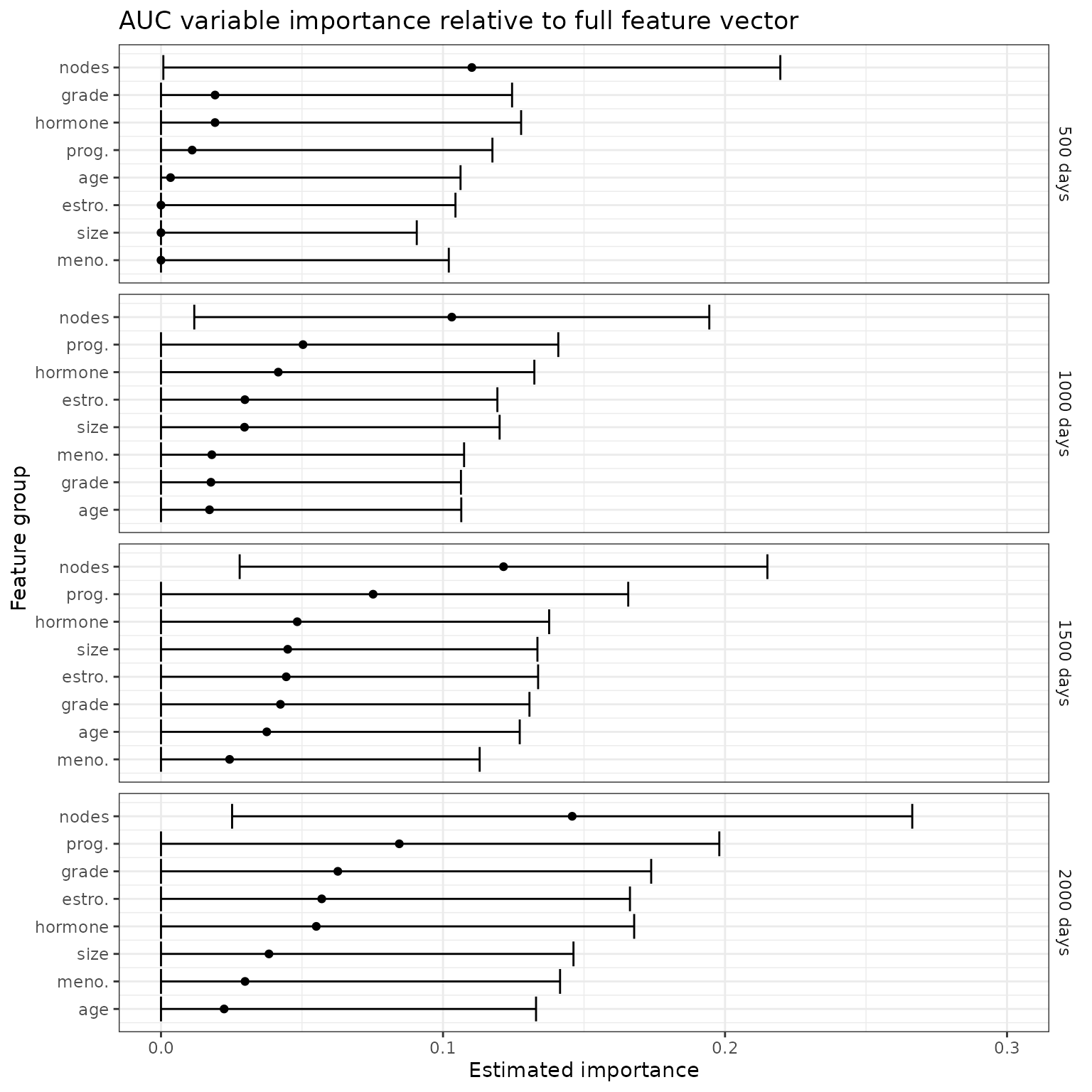

# repeat the analysis for feature groups
for (i in 1:length(feature_group_names2)){
  indx_char <- feature_groups2[i]
  indx_name <- feature_group_names2[i]
  indx <- as.numeric(strsplit(indx_char, split = ",")[[1]])
  
  reduced_preds <- crossfit_oracle_preds(time = time,
                                         event = event,
                                         X = X,
                                         folds = folds,
                                         nuisance_preds = augmented_nuisance_preds,
                                         pred_generator = generate_reduced_oracle_predictions,
                                         landmark_times = landmark_times,
                                         approx_times = approx_times,
                                         SL.library = SL.library,
                                         indx = indx)
  CV_reduced_preds <- reduced_preds$oracle_preds
  
  output <- vim_AUC(time = time,
                    event = event,
                    approx_times = approx_times,
                    landmark_times = landmark_times,
                    f_hat = lapply(CV_full_preds, function(x) 1-x),
                    fs_hat = lapply(CV_reduced_preds, function(x) 1-x),
                    S_hat = CV_S_preds,
                    G_hat = CV_G_preds,
                    folds = folds,
                    ss_folds = ss_folds,
                    sample_split = TRUE,
                    scale_est = TRUE)

  output$vim <- "AUC"
  output$indx <- rep(indx_char, nrow(output))
  output$indx_name <- rep(indx_name, nrow(output))
  if (!(i == 1)){
    pooled_output <- rbind(pooled_output, output)
  } else{
    pooled_output <- output
  }
}

p_auc <- pooled_output %>%
  mutate(landmark_time = factor(landmark_time,
                                levels = c(500, 1000, 1500, 2000),
                                labels = c("500 days", "1000 days", "1500 days", "2000 days"))) %>%
  arrange(landmark_time, est) %>%
  mutate(Order = row_number()) %>%
  {ggplot(., aes(x = est, y = Order)) +
      geom_errorbarh(aes(xmin = cil, xmax = ciu)) +
      geom_point() +
      theme_bw() +
      xlab("Estimated importance") +
      ylab("Feature group") +
      xlim(c(0,0.5)) +
      scale_y_continuous(
        breaks = .$Order,
        labels = .$indx_name,
      ) +
      facet_wrap(~landmark_time, dir = "v", strip.position = "right", scales = "free_y", ncol = 1) +
      ggtitle("AUC variable importance relative to full feature vector (groups)")+
      theme(strip.background = element_blank(),
            strip.placement = "outside")
  }
p_auc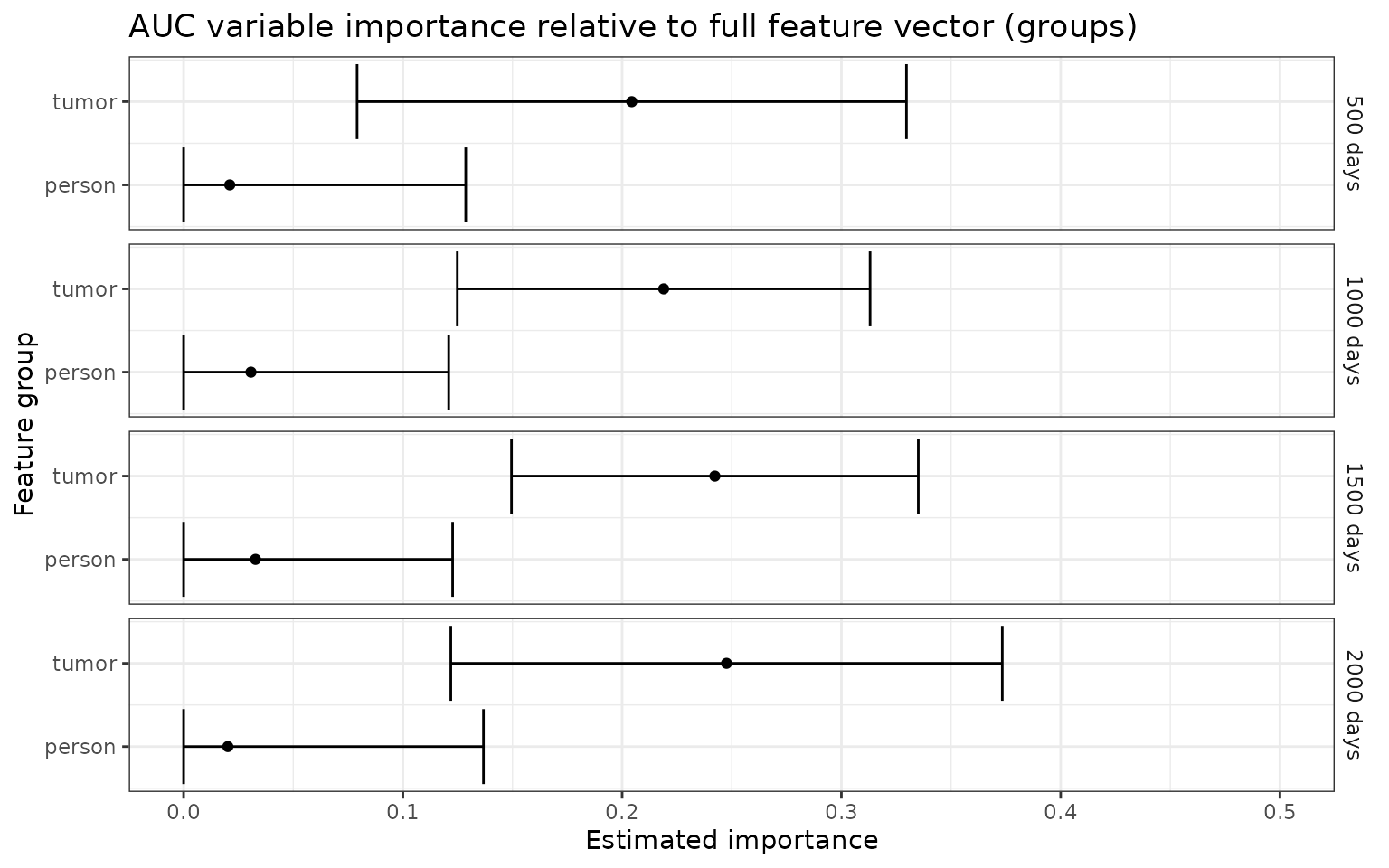

Estimating variable importance relative to base model

Next, we consider the importance of each of the tumor-level features relative to a baseline set of person-level features. Here, the feature of interest is added to a baseline set of features, with importance measured by the resulting gain in predictiveness.

For this analysis, the “full” oracle predictions include baseline features plus the feature of interest, and the “residual” oracle predictions include only baseline features. Note that both the full and residual oracle prediction functions for this analysis are estimated by regressing the conditional survival function estimates given all features on the relevant reduced feature set. As in the previous analysis, this step is necessary to account for censoring that may be informed by covariates, even those which are not included in the current set of predictors.

# For importance relative to baseline features, the "reduced" model uses only person-level (baseline) features
# The "full" model uses baseline + feature of interest
# We wrote generate_reduced_predictions() to leave out the "indx" argument. Need to keep that in mind!
size_index <- paste0(c(size_index, person_index), collapse = ",")
nodes_index <- paste0(c(nodes_index, person_index), collapse = ",")
pgr_index <- paste0(c(pgr_index, person_index), collapse = ",")
er_index <- paste0(c(er_index, person_index), collapse = ",")
grade_index <- paste0(c(grade_index, person_index), collapse = ",")

feature_group_names <- c("size", "nodes", "prog.", "estro.", "grade")
feature_groups <- c(size_index, nodes_index,
                    pgr_index, er_index, grade_index)

reduced_preds <- crossfit_oracle_preds(time = time,
                                       event = event,
                                       X = X,
                                       folds = folds,
                                       nuisance_preds = augmented_nuisance_preds,
                                       pred_generator = generate_reduced_oracle_predictions,
                                       landmark_times = landmark_times,
                                       approx_times = approx_times,
                                       SL.library = SL.library,
                                       indx = as.numeric(strsplit(tum_index, split = ",")[[1]]))
CV_reduced_preds <- reduced_preds$oracle_preds

for (i in 1:length(feature_group_names)){
  indx_char <- feature_groups[i]
  indx_name <- feature_group_names[i]
  indx <- as.numeric(strsplit(indx_char, split = ",")[[1]])
  
  all_indx <- 1:ncol(X)
  # leave out features *not* in indx for this analysis
  indx <- all_indx[-which(all_indx %in% indx)]
  
  full_preds <- crossfit_oracle_preds(time = time,
                                      event = event,
                                      X = X,
                                      folds = folds,
                                      nuisance_preds = augmented_nuisance_preds,
                                      pred_generator = generate_reduced_oracle_predictions,
                                      landmark_times = landmark_times,
                                      approx_times = approx_times,
                                      SL.library = SL.library,
                                      indx = indx)
  CV_full_preds <- full_preds$oracle_preds
  
  output <- vim_AUC(time = time,
                    event = event,
                    approx_times = approx_times,
                    landmark_times = landmark_times,
                    f_hat = lapply(CV_full_preds, function(x) 1-x),
                    fs_hat = lapply(CV_reduced_preds, function(x) 1-x),
                    S_hat = CV_S_preds,
                    G_hat = CV_G_preds,
                    folds = folds,
                    ss_folds = ss_folds,
                    sample_split = TRUE,
                    scale_est = TRUE)
  
  output$vim <- "AUC"
  output$indx <- rep(indx_char, nrow(output))
  output$indx_name <- rep(indx_name, nrow(output))
  if (!(i == 1)){
    pooled_output <- rbind(pooled_output, output)
  } else{
    pooled_output <- output
  }
}

p_auc <- pooled_output %>%
    mutate(landmark_time = factor(landmark_time,
                                levels = c(500, 1000, 1500, 2000),
                                labels = c("500 days", "1000 days", "1500 days", "2000 days"))) %>%
  arrange(landmark_time, est) %>%
  mutate(Order = row_number()) %>%
  {ggplot(., aes(x = est, y = Order)) +
      geom_errorbarh(aes(xmin = cil, xmax = ciu)) +
      geom_point() +
      theme_bw() +
      xlab("Estimated importance") +
      ylab("Feature group") +
      xlim(c(0,0.4)) +
      scale_y_continuous(
        breaks = .$Order,
        labels = .$indx_name,
      ) + 
      facet_wrap(~landmark_time, dir = "v", strip.position = "right", scales = "free_y", ncol = 1) + 
      ggtitle("AUC variable importance relative to person-level features")+
      theme(strip.background = element_blank(),
            strip.placement = "outside")#,
  }
p_auc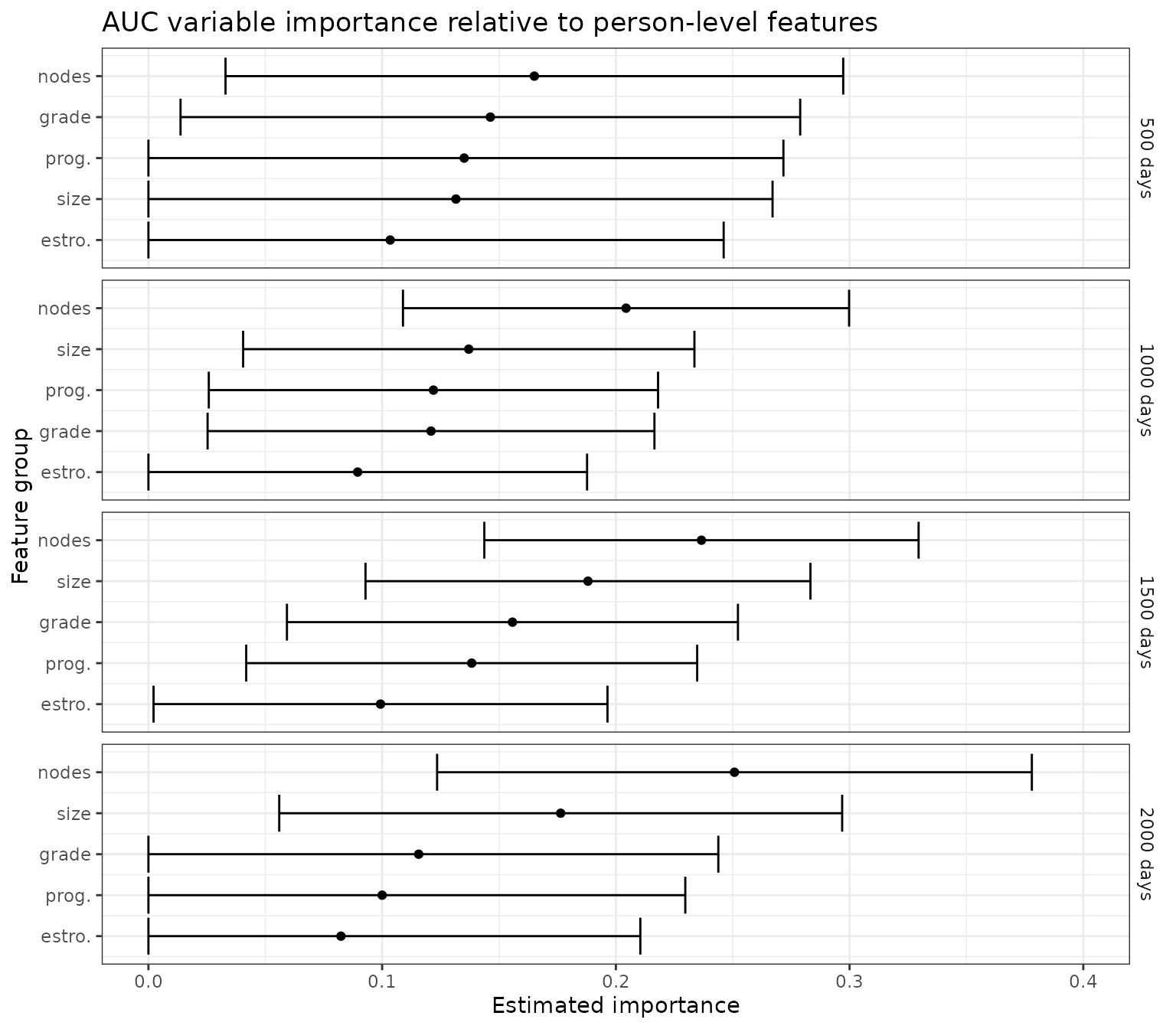

Adjustment variables

There may be covariates that are thought to influence both $T$ and $C$ but are not of scientific interest in terms of variable importance. (We may think of these covariates as analogous to confounders in a causal inference setting.) It is important to adjust for these variables in all analyses. In the gbsg analysis, for example, we may wish to adjust for person-level covariates age, menopausal status, and hormone treatment therapy, but to assess variable importance using only the predictiveness of tumor-level covariates.

We use $r$ to denote the index set of adjustment variables, and again use $s$ to denote the index set of variables of interest. The importance of $X_s$ relative to $X_{-r}$ (i.e., the full covariate vector excluding adjustment variables) is given by $V(f_{0, r}, P_0) - V(f_{0, (r \cup s)}, P_0)$.

As usual, there are many possible approaches to estimating $f_{0,r}$ and $f_{0,(r \cup s)}$, depending on their explicit form. In the case of AUC predictiveness, we can simply estimate the prediction models $f_{0,r}$ and $f_{0,(r \cup s)}$ by (1) estimating the full oracle prediction function $f_0$, (2) generating predictions for individuals in the training data, and then (3) regressing those predictions on the appropriate reduced covariate vector.

Here, we analyze VIM relative to tumor-level covariates, while adjusting for person-level covariates.

size_index <- paste0(c(size_index, person_index), collapse = ",")
nodes_index <- paste0(c(nodes_index, person_index), collapse = ",")
pgr_index <- paste0(c(pgr_index, person_index), collapse = ",")
er_index <- paste0(c(er_index, person_index), collapse = ",")
grade_index <- paste0(c(grade_index, person_index), collapse = ",")

feature_group_names <- c("size", "nodes", "prog.", "estro.", "grade")
feature_groups <- c(size_index, nodes_index,
                    pgr_index, er_index, grade_index)

# in this analysis, "full" predictions are obtained by regressing the conditional survival
# function estimates given all features on the tumor-level features, i.e., leaving out
# person features
full_preds <- crossfit_oracle_preds(time = time,
                                    event = event,
                                    X = X,
                                    folds = folds,
                                    nuisance_preds = augmented_nuisance_preds,
                                    pred_generator = generate_reduced_oracle_predictions,
                                    landmark_times = landmark_times,
                                    approx_times = approx_times,
                                    SL.library = SL.library,
                                    indx = as.numeric(strsplit(person_index, split = ",")[[1]]))
CV_full_preds <- full_preds$oracle_preds

for (i in 1:length(feature_group_names)){
  indx_char <- feature_groups[i]
  indx_name <- feature_group_names[i]
  indx <- as.numeric(strsplit(indx_char, split = ",")[[1]])
  
  reduced_preds <- crossfit_oracle_preds(time = time,
                                         event = event,
                                         X = X,
                                         folds = folds,
                                         nuisance_preds = augmented_nuisance_preds,
                                         pred_generator = generate_reduced_oracle_predictions,
                                         landmark_times = landmark_times,
                                         approx_times = approx_times,
                                         SL.library = SL.library,
                                         indx = indx)
  CV_reduced_preds <- reduced_preds$oracle_preds

  output <- vim_AUC(time = time,
                    event = event,
                    approx_times = approx_times,
                    landmark_times = landmark_times,
                    f_hat = lapply(CV_full_preds, function(x) 1-x),
                    fs_hat = lapply(CV_reduced_preds, function(x) 1-x),
                    S_hat = CV_S_preds,
                    G_hat = CV_G_preds,
                    folds = folds,
                    ss_folds = ss_folds,
                    sample_split = TRUE,
                    scale_est = TRUE)
  
  output$vim <- "AUC"
  output$indx <- rep(indx_char, nrow(output))
  output$indx_name <- rep(indx_name, nrow(output))
  if (!(i == 1)){
    pooled_output <- rbind(pooled_output, output)
  } else{
    pooled_output <- output
  }
}

p_auc <- pooled_output %>%
    mutate(landmark_time = factor(landmark_time,
                                levels = c(500, 1000, 1500, 2000),
                                labels = c("500 days", "1000 days", "1500 days", "2000 days"))) %>%
  arrange(landmark_time, est) %>%
  mutate(Order = row_number()) %>%
  {ggplot(., aes(x = est, y = Order)) +
      geom_errorbarh(aes(xmin = cil, xmax = ciu)) +
      geom_point() +
      theme_bw() +
      xlab("Estimated importance") +
      ylab("Feature group") +
      xlim(c(0,0.4)) +
      scale_y_continuous(
        breaks = .$Order,
        labels = .$indx_name,
      ) + 
      facet_wrap(~landmark_time, dir = "v", strip.position = "right", scales = "free_y", ncol = 1) + 
      ggtitle("Adjusted AUC variable importance relative to all tumor-level features")+
      theme(strip.background = element_blank(),
            strip.placement = "outside")#,
  }
p_auc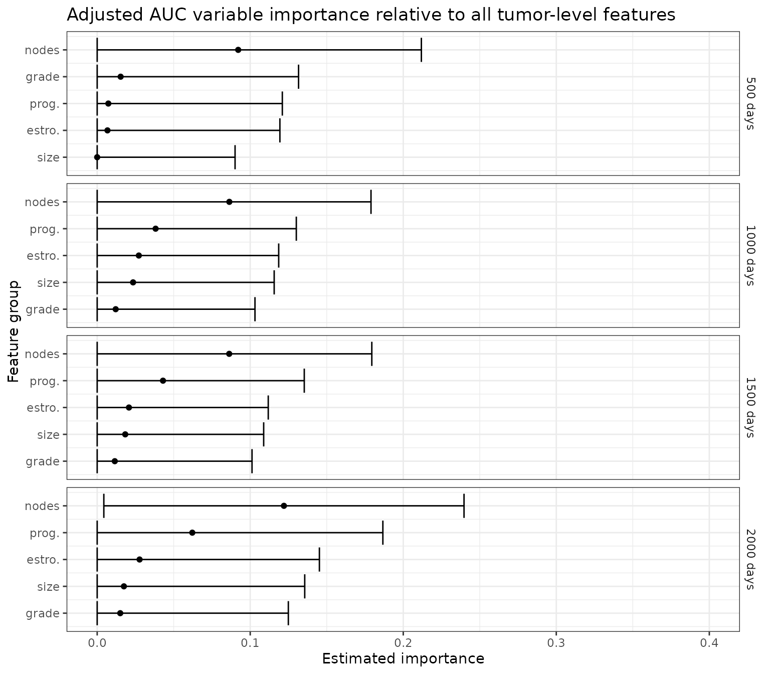

Doubly-robust estimation

The VIM estimation procedure implemented in survML is doubly-robust with respect to the conditional time-to-event survival function $S_0$ and conditional censoring survival function $G_0$: Roughly speaking, as long as one of these two nuisance functions is estimated well, the VIM estimator will tend in probability to the true population VIM as the sample size increases.

In many cases, the oracle prediction functions $f_0$ and $f_{0,s}$ can themselves be estimated in a doubly-robust manner. For example, for AUC and Brier score VIMs evaluated at landmark time $\tau$, the oracle prediction function is simply $S_0(\tau \mid x)$. The pseudo-outcome approach of Rubin and van der Laan (2007) can be used to construct a doubly-robust estimator of a conditional survival function at a single time-point, at the computational cost of performing an additional regression step. Given initial estimates of $S_0$ and $G_0$, the following code constructs a doubly-robust estimate of $S_0(\tau \mid x)$ using Super Learner.

generate_full_oracle_predictions_DR <- function(time,
                                                event,
                                                X,
                                                X_holdout,
                                                nuisance_preds,
                                                landmark_times,
                                                approx_times,
                                                SL.library){
  
  S_hat <- nuisance_preds$S_preds_train
  G_hat <- nuisance_preds$G_preds_train
  
  DR_predictions_combined <- DR_pseudo_outcome_regression(time = time,
                                                          event = event,
                                                          X = X,
                                                          newX = rbind(X_holdout, X),
                                                          S_hat = S_hat,
                                                          G_hat = G_hat,
                                                          newtimes = landmark_times,
                                                          approx_times = approx_times,
                                                          SL.library = SL.library)
  
  DR_predictions <- DR_predictions_combined[1:nrow(X_holdout),]
  DR_predictions_train <- DR_predictions_combined[(nrow(X_holdout) + 1):nrow(DR_predictions_combined),]

  return(list(f0_hat = DR_predictions,
              f0_hat_train = DR_predictions_train))
  
}

This doubly-robust estimator of $f_0$ can then be regressed on the reduced covariate vector to give a doubly-robust estimator of $f_{0,s}$. These doubly-robust estimated oracle prediction functions can be used in the usual manner to estimate variable importance. Here, we repeat the original analysis using the doubly-robust pseudo-outcome approach.

# reset feature groups
age_index <- paste0(which(X_names == "age"))
meno_index <- paste0(which(X_names == "meno"))
size_index <- paste0(which(X_names == "size"))
nodes_index <- paste0(which(X_names == "nodes"))
pgr_index <- paste0(which(X_names == "pgr"))
er_index <- paste0(which(X_names == "er"))
hormon_index <- paste0(which(X_names == "hormon"))
grade_index <- paste0(which(X_names %in% c("tumgrad2", "tumgrad3")), collapse = ",")

feature_group_names <- c("age", "meno.", "size", "nodes",
                         "prog.", "estro.", "hormone", 
                         "grade")
feature_groups <- c(age_index, meno_index, size_index, nodes_index,
                    pgr_index, er_index, hormon_index, grade_index)

# generate full oracle estimates
full_preds <- crossfit_oracle_preds(time = time,
                                    event = event,
                                    X = X,
                                    folds = folds,
                                    nuisance_preds = nuisance_preds,
                                    pred_generator = generate_full_oracle_predictions_DR,
                                    landmark_times = landmark_times,
                                    approx_times = approx_times,
                                    SL.library = SL.library)

CV_full_preds <- full_preds$oracle_preds
CV_full_preds_train <- full_preds$oracle_preds_train

augmented_nuisance_preds <- nuisance_preds
augmented_nuisance_preds$full_preds_train <- CV_full_preds_train

# iterate over feature groups
for (i in 1:length(feature_group_names)){
  indx_char <- feature_groups[i]
  indx_name <- feature_group_names[i]
  indx <- as.numeric(strsplit(indx_char, split = ",")[[1]])
  
  # estimate residual oracle prediction function for this feature group
  reduced_preds <- crossfit_oracle_preds(time = time,
                                         event = event,
                                         X = X,
                                         folds = folds,
                                         nuisance_preds = augmented_nuisance_preds,
                                         pred_generator = generate_reduced_oracle_predictions,
                                         landmark_times = landmark_times,
                                         approx_times = approx_times,
                                         SL.library = SL.library,
                                         indx = indx)
  CV_reduced_preds <- reduced_preds$oracle_preds

  # estimate VIM - note the oracle for AUC is the conditional cdf, not survival function, 
  # so need to take 1 - S(tau | x)
  output <- vim_AUC(time = time,
                    event = event,
                    approx_times = approx_times,
                    landmark_times = landmark_times,
                    f_hat = lapply(CV_full_preds, function(x) 1-x),
                    fs_hat = lapply(CV_reduced_preds, function(x) 1-x),
                    S_hat = CV_S_preds,
                    G_hat = CV_G_preds,
                    folds = folds,
                    ss_folds = ss_folds,
                    sample_split = TRUE,
                    scale_est = TRUE)
  
  output$vim <- "AUC"
  output$indx <- rep(indx_char, nrow(output))
  output$indx_name <- rep(indx_name, nrow(output))
  if (!(i == 1)){
    pooled_output <- rbind(pooled_output, output)
  } else{
    pooled_output <- output
  }
}

# plot results
p_auc <- pooled_output %>%
   mutate(landmark_time = factor(landmark_time,
                                levels = c(500, 1000, 1500, 2000),
                                labels = c("500 days", "1000 days", "1500 days", "2000 days"))) %>%
  arrange(landmark_time, est) %>%
  mutate(Order = row_number()) %>%
  {ggplot(., aes(x = est, y = Order)) +
      geom_errorbarh(aes(xmin = cil, xmax = ciu)) +
      geom_point() +
      theme_bw() +
      xlab("Estimated importance") +
      ylab("Feature group") +
      xlim(c(0,0.3)) +
      scale_y_continuous(
        breaks = .$Order,
        labels = .$indx_name,
      ) + 
      facet_wrap(~landmark_time, dir = "v", strip.position = "right", scales = "free_y", ncol = 1) + 
      ggtitle("AUC variable importance relative to all features (doubly-robust pseudo-outcome)")+
      theme(strip.background = element_blank(),
            strip.placement = "outside")
  }
p_auc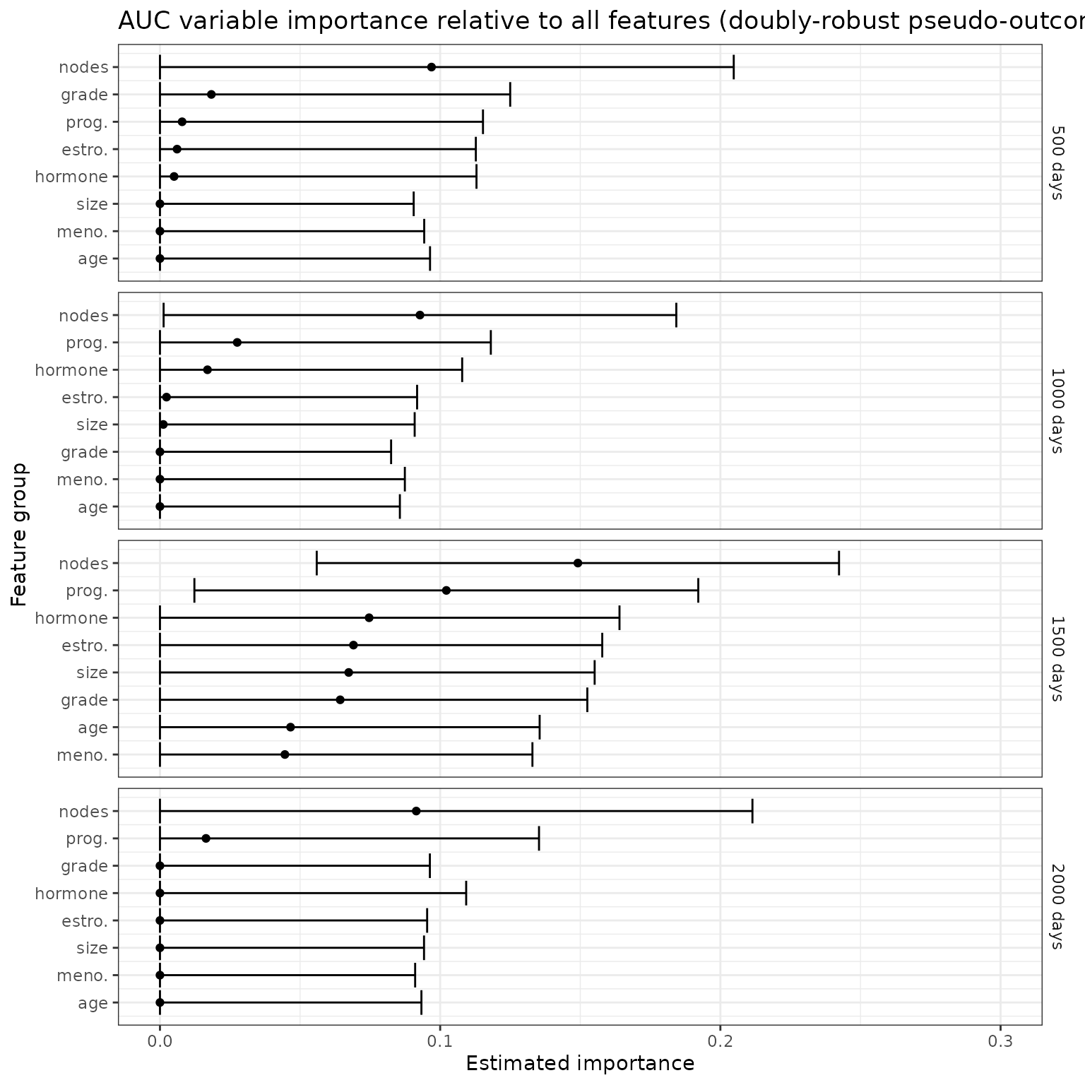

Appendix

Some example predictiveness measures, along with the corresponding oracle prediction functions, are given below.

• AUC:
  • $V(f, P_0) = P_0\{f(X_1) > f(X_2) \mid T_1 \leq \tau, T_2 > \tau\}$
  • $f_0(x) = 1 - S_0(\tau \mid x)$
• Brier score:
  • $V(f, P_0) = E_{P_0}[\{f(X) - I(T > \tau)\}^2]$
  • $f_0(x) = S_0(\tau \mid x)$
• Survival time MSE:
  • $V(f, P_0) = E_{P_0}[\{f(X) - (T \wedge \tau)\}^2]$
  • $f_0(x) = \int_0^\tau S_0(t \mid x)dt$
• Proportion of explained variance:
  • $V(f, P_0) = \frac{E_{P_0}[\{f(X) - I(T > \tau)\}^2]}{var[I(T > \tau)]}$
  • $f_0(x) = S_0(\tau \mid x)$
• Binary classification accuracy:
  • $V(f, P_0) = P_0\{f(X) = I(T > \tau)\}$
  • $f_0(x) = I\{S_0(\tau \mid x) > 0.5\}$
• C-index:
  • $V(f, P_0) = P_0\{f(X_1) > f(X_2) \mid T_1 \leq T_2\}$
  • For the C-index, there is, to our knowledge, no closed form of the oracle prediction function; see the preprint for more details on our proposed procedure for direct numerical optimization.

References

The survival variable importance methodology is described in

Charles J. Wolock, Peter B. Gilbert, Noah Simon and Marco Carone. “Assessing variable importance in survival analysis using machine learning.” arXiv:2311.12726.

Other references:

David R. Cox. “Regression Models and Life-Tables.” Journal of the Royal Statistical Society: Series B (Methodological) (1972).

Ted Westling, Alex Luedtke, Peter B. Gilbert and Marco Carone. “Inference for treatment-specific survival curves using machine learning.” Journal of the American Statistical Association (2023).

Charles J. Wolock, Peter B. Gilbert, Noah Simon and Marco Carone. “A framework for leveraging machine learning tools to estimate personalized survival curves.” Journal of Computational and Graphical Statistics (2024).

Mark J. van der Laan, Eric C. Polley and Alan E. Hubbard. “Super learner”. Statistical Applications in Genetics and Molecular Biology (2007).

Daniel Rubin and Mark J. van der Laan. “A doubly robust censoring unbiased transformation”. International Journal of Biostatistics (2007).