Estimating a conditional survival function using off-the-shelf machine learning tools • survML

library(survML)
#> Loading required package: SuperLearner
#> Loading required package: nnls
#> Loading required package: gam
#> Loading required package: splines
#> Loading required package: foreach
#> Loaded gam 1.22-5
#> Super Learner
#> Version: 2.0-29
#> Package created on 2024-02-06
library(ggplot2)
library(gam)

Introduction

The survML package implements two methods for estimating a conditional survival function using off-the-shelf machine learning. The first, called global survival stacking and performed using the stackG() function, involves decomposing the conditional cumulative hazard function into regression functions depending only on the observed data. The second, called local survival stacking or discrete-time hazard estimation, involves discretizing time and estimating the probability of an event of interest within each discrete time period. This procedure is implemented in the stackL() function.

These functions can be used for both left-truncated, right-censored data (commonly seen in prospective studies) and right-truncated data (commonly seen in retrospective studies).

More details on each method, as well as examples, follow.

Global survival stacking

In a basic survival analysis setting with right-censored data (for simplicity, we don’t discuss truncation here), the ideal data for each individual consist of a covariate vector $X$ , an event time $T$ , and a censoring time $C$ . The observed data consist of $X$ , the observed follow-up time $Y:=\text{min}(T,C)$ , and the event indicator $\Delta := I(T \leq C)$ . Global survival stacking requires three components: (1) the conditional probability that $\Delta = 1$ given $X$ , (2) the CDF of $Y$ given $X$ among among censored subjects, and (3) the CDF of $Y$ given $X$ among uncensored subjects. All three of these can be estimated using standard binary regression or classification methods.

Estimating (1) is a standard binary regression problem. We use pooled binary regression to estimate (2) and (3). In essence, at time $t$ each on a user-specified grid, the CDF is a binary regression using the outcome $I(Y \leq t)$ . The data sets for each $t$ are combined into a single, pooled data set, including $t$ as a covariate. Currently, survML allows Super Learner to be used for binary regression, but more learners will be added in future versions.

The stackG function performs global survival stacking. The most important user-specified arguments are described here:

bin_size: This is the size of time grid used for estimating (2) and (3). In most cases, a finer grid performs better than a coarser grid, at increased computational cost. We recommend using as fine a grid as computational resources and time allow. In simulations, a grid of 40 time points performed similarly to a grid of every observed follow-up time. Bin size is given in quantile terms; bin_size = 0.025 will use times corresponding to quantiles $\{0, 0.025, 0.05, \dots, 0.975, 1\}$ . If NULL, a grid of every observed time is used.
time_basis: This is how the time variable $t$ is included in the pooled data set. The default is continuous (i.e., include time as-is). It is also possible to include a dummy variable for each time in the grid (i.e., treat time as a factor variable) using option dummy.
learner: Currently, the only supported option is SuperLearner.
SL_control: This is a named list of arguments that are passed directly to the SuperLearner() function. SL.library gives the library of algorithms to be included in the Super Learner binary regression. This argument should be vector of algorithm names, which can be either default algorithms included in the SuperLearner package, or user-specified algorithms. See the SuperLearner package documentation for more information.
time_grid_approx: This is the grid of times used to approximate the cumulative hazard or product integral. While this argument defaults to a grid of every observed follow-up time, this can have a substantial computational cost in large samples. Using a coarser grid (e.g., of ~100 time points) will decrease runtime and usually has little impact on performance.

Example

Here’s a small example applying stackG to simulated data.

# This is a small simulation example
set.seed(123)
n <- 500
X <- data.frame(X1 = rnorm(n), X2 = rbinom(n, size = 1, prob = 0.5))

S0 <- function(t, x){
  pexp(t, rate = exp(-2 + x[,1] - x[,2] + .5 * x[,1] * x[,2]), lower.tail = FALSE)
}
T <- rexp(n, rate = exp(-2 + X[,1] - X[,2] + .5 *  X[,1] * X[,2]))

G0 <- function(t, x) {
  as.numeric(t < 15) *.9*pexp(t,
                              rate = exp(-2 -.5*x[,1]-.25*x[,2]+.5*x[,1]*x[,2]),
                              lower.tail=FALSE)
}
C <- rexp(n, exp(-2 -.5 * X[,1] - .25 * X[,2] + .5 * X[,1] * X[,2]))
C[C > 15] <- 15

time <- pmin(T, C)
event <- as.numeric(T <= C)

# note that this a very small library, just for demonstration
SL.library <- c("SL.mean", "SL.glm", "SL.gam")

fit <- stackG(time = time,
              event = event,
              X = X,
              newX = X,
              newtimes = seq(0, 15, .1),
              direction = "prospective",
              bin_size = 0.1,
              time_basis = "continuous",
              time_grid_approx = sort(unique(time)),
              surv_form = "exp",
              SL_control = list(SL.library = SL.library,
                                V = 5))

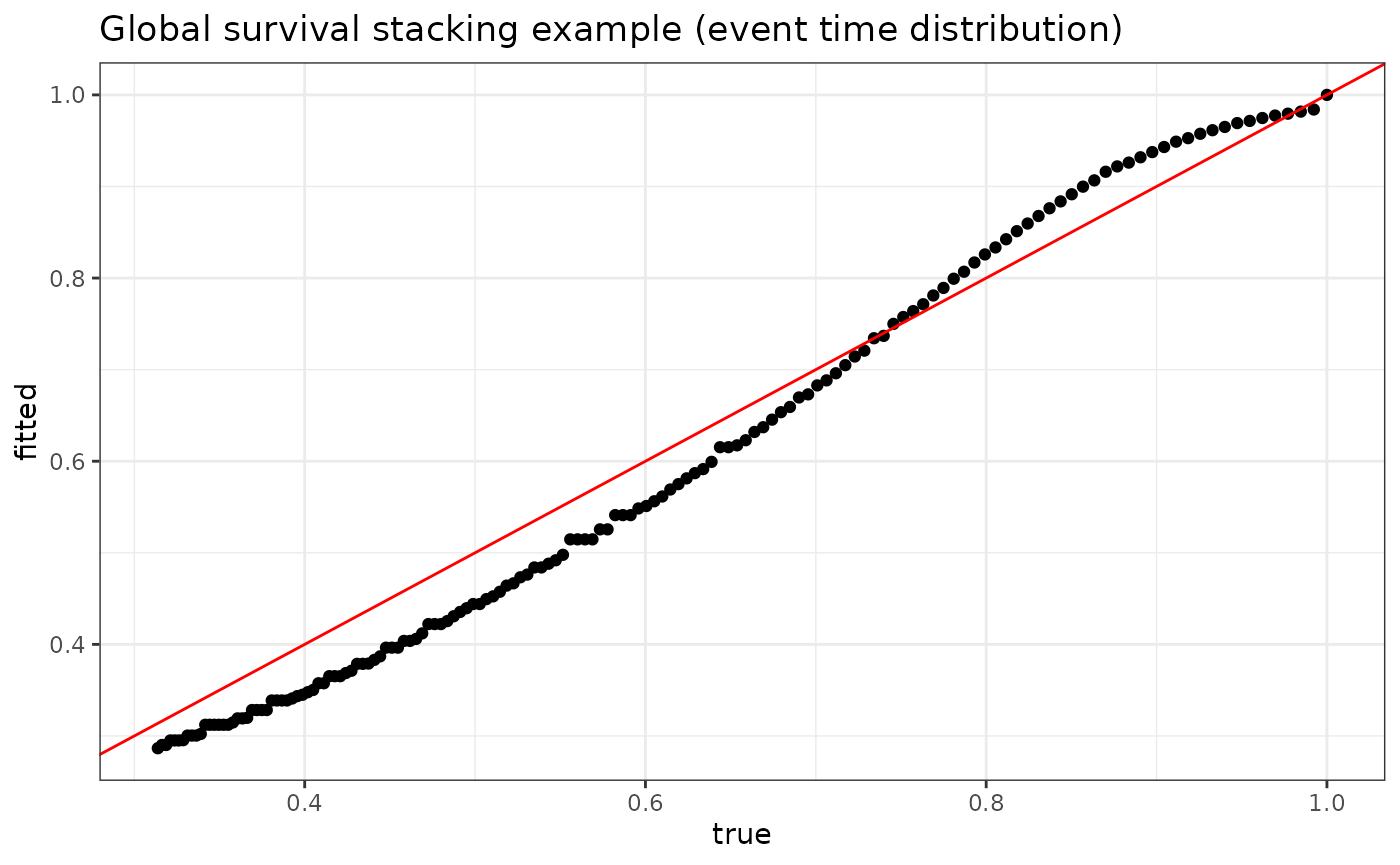
We can plot the fitted versus true conditional survival at various times for one particular individual in our data set:

plot_dat <- data.frame(fitted = fit$S_T_preds[1,], 
                       true = S0(t =  seq(0, 15, .1), X[1,]))

p <- ggplot(data = plot_dat, mapping = aes(x = true, y = fitted)) + 
  geom_point() + 
  geom_abline(slope = 1, intercept = 0, color = "red") + 
  theme_bw() + 
  ylab("fitted") +
  xlab("true") + 
  ggtitle("Global survival stacking example (event time distribution)")

p

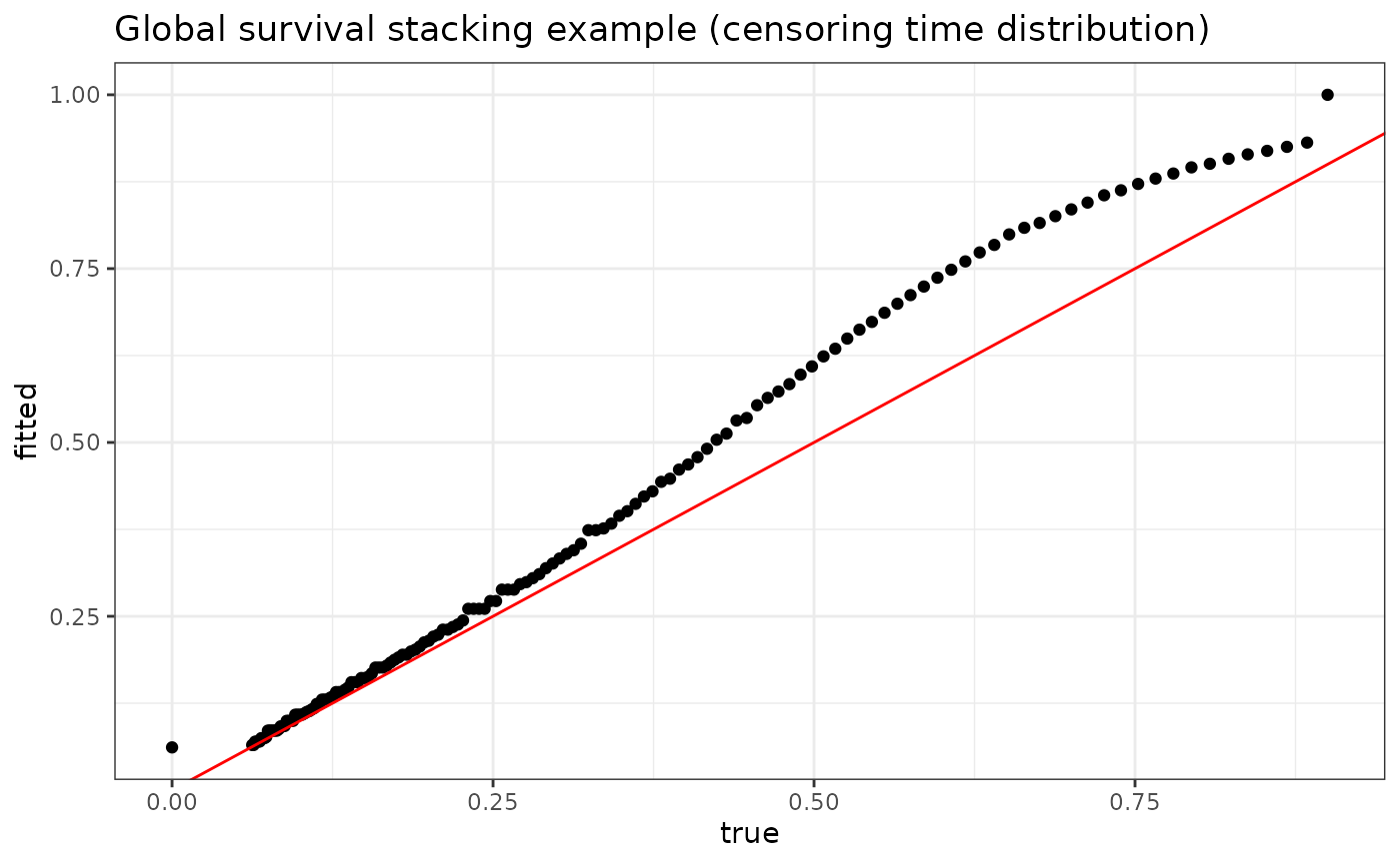
The stackG function simultaneously produces estimates for the conditional censoring distribution. This may be useful, for example, for producing inverse probability of censoring (IPCW) weights.

plot_dat <- data.frame(fitted = fit$S_C_preds[1,], 
                       true = G0(t =  seq(0, 15, .1), X[1,]))

p <- ggplot(data = plot_dat, mapping = aes(x = true, y = fitted)) + 
  geom_point() + 
  geom_abline(slope = 1, intercept = 0, color = "red") + 
  theme_bw() + 
  ylab("fitted") +
  xlab("true") + 
  ggtitle("Global survival stacking example (censoring time distribution)")

p

Local survival stacking

For discrete time-to-event variables, the hazard function at a single time is a conditional probability whose estimation can be framed as a binary regression problem: among those who have not experienced the event by time $t$ , what proportion experience the outcome at that time? Local survival stacking assumes a discrete survival process and is based on estimating this conditional event probability at each time in a user-specified grid. These binary regressions are estimated jointly by “stacking” the data sets corresponding to all times in the grid. This idea dates back at least to work by Polley and van der Laan (2011) and was also recently described by Craig et al. (2021).

Example

fit <- stackL(time = time,
              event = event,
              X = X,
              newX = X,
              newtimes = seq(0, 15, .1),
              direction = "prospective",
              bin_size = 0.1,
              time_basis = "continuous",
              SL_control = list(SL.library = SL.library,
                                V = 5))

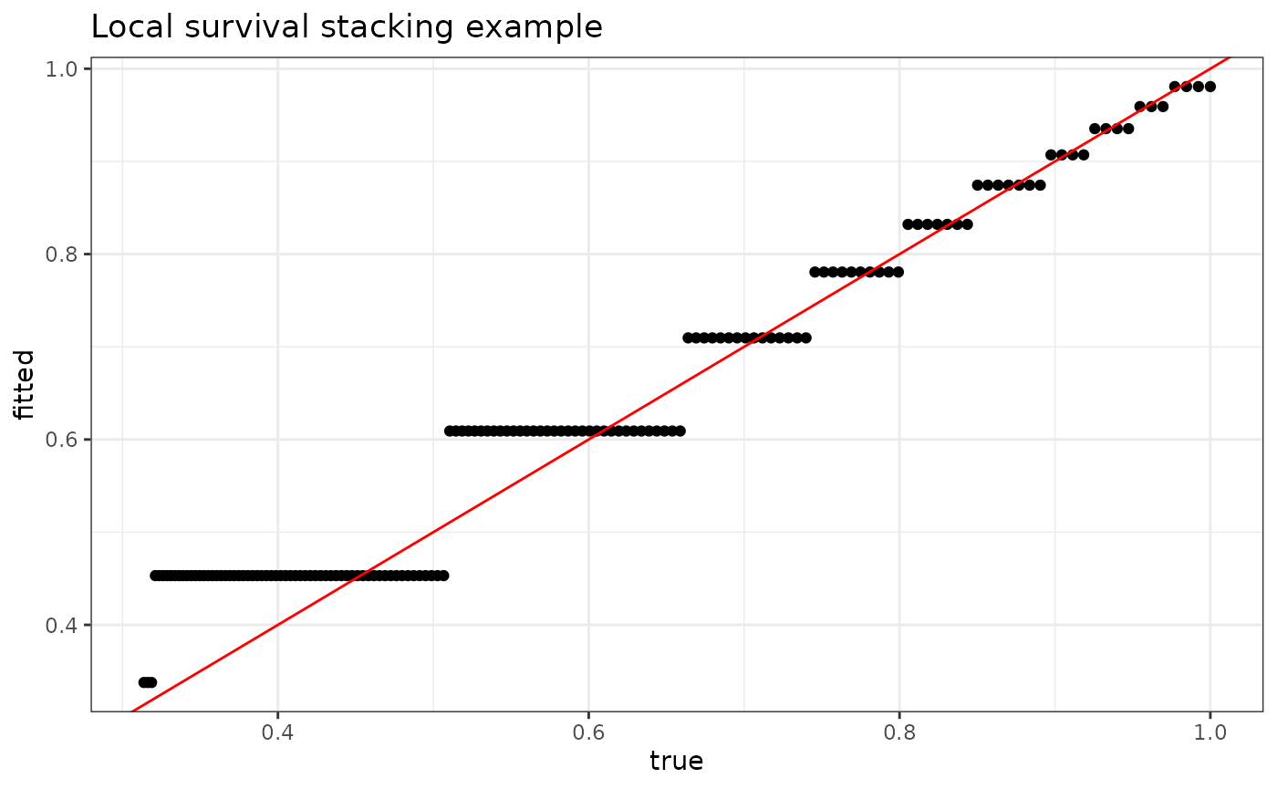
plot_dat <- data.frame(fitted = fit$S_T_preds[1,], 
                       true = S0(t =  seq(0, 15, .1), X[1,]))

p <- ggplot(data = plot_dat, mapping = aes(x = true, y = fitted)) + 
  geom_point() + 
  geom_abline(slope = 1, intercept = 0, color = "red") + 
  theme_bw() + 
  ylab("fitted") +
  xlab("true") + 
  ggtitle("Local survival stacking example")

p

References

For details of global survival stacking, please see the following paper:

Charles J. Wolock, Peter B. Gilbert, Noah Simon and Marco Carone. “A framework for leveraging machine learning tools to estimate personalized survival curves.” Journal of Computational and Graphical Statistics (2024).

Local survival stacking is described in:

Eric C. Polley and Mark J. van der Laan. “Super Learning for Right-Censored Data.” In Targeted Learning (2011).

Erin Craig, Chenyang Zhong, and Robert Tibshirani. “Survival stacking: casting survival analysis as a classification problem.” arXiv:2107.13480 (2021).