Estimate a conditional survival function using global survival stacking

Usage

stackG(
  time,
  event = rep(1, length(time)),
  entry = NULL,
  X,
  newX = NULL,
  newtimes = NULL,
  direction = "prospective",
  time_grid_fit = NULL,
  bin_size = NULL,
  time_basis,
  time_grid_approx = sort(unique(time)),
  surv_form = "PI",
  learner = "SuperLearner",
  SL_control = list(SL.library = c("SL.mean"), V = 10, method = "method.NNLS", stratifyCV
    = FALSE),
  tau = NULL
)

Arguments

time: n x 1 numeric vector of observed follow-up times If there is censoring, these are the minimum of the event and censoring times.
event: n x 1 numeric vector of status indicators of whether an event was observed. Defaults to a vector of 1s, i.e. no censoring.
entry: Study entry variable, if applicable. Defaults to NULL, indicating that there is no truncation.
X: n x p data.frame of observed covariate values on which to train the estimator.
newX: m x p data.frame of new observed covariate values at which to obtain m predictions for the estimated algorithm. Must have the same names and structure as X.
newtimes: k x 1 numeric vector of times at which to obtain k predicted conditional survivals.
direction: Whether the data come from a prospective or retrospective study. This determines whether the data are treated as subject to left truncation and right censoring ("prospective") or right truncation alone ("retrospective").
time_grid_fit: Named list of numeric vectors of times of times on which to discretize for estimation of cumulative probability functions. This is an alternative to bin_size and allows for specially tailored time grids rather than simply using a quantile bin size. The list consists of vectors named F_Y_1_grid, F_Y_0_grid, G_W_1_grid, and G_W_0_grid. These denote, respectively, the grids used to estimate the conditional CDF of the time variable among uncensored and censored observations, and the grids used to estimate the conditional distribution of the entry variable among uncensored and censored observations.
bin_size: Size of time bin on which to discretize for estimation of cumulative probability functions. Can be a number between 0 and 1, indicating the size of quantile grid (e.g. 0.1 estimates the cumulative probability functions on a grid based on deciles of observed times). If NULL, creates a grid of all observed times.
time_basis: How to treat time for training the binary classifier. Options are "continuous" and "dummy", meaning an indicator variable is included for each time in the time grid.
time_grid_approx: Numeric vector of times at which to approximate product integral or cumulative hazard interval. Defaults to times argument.
surv_form: Mapping from hazard estimate to survival estimate. Can be either "PI" (product integral mapping) or "exp" (exponentiated cumulative hazard estimate).
learner: Which binary regression algorithm to use. Currently, only SuperLearner is supported, but more learners will be added. See below for algorithm-specific arguments.
SL_control: Named list of parameters controlling the Super Learner fitting process. These parameters are passed directly to the SuperLearner function. Parameters include SL.library (library of algorithms to include in the binary classification Super Learner), V (Number of cross validation folds on which to train the Super Learner classifier, defaults to 10), method (Method for estimating coefficients for the Super Learner, defaults to "method.NNLS"), stratifyCV (logical indicating whether to stratify by outcome in SuperLearner's cross-validation scheme), and obsWeights (observation weights, passed directly to prediction algorithms by SuperLearner).
tau: The maximum time of interest in a study, used for retrospective conditional survival estimation. Rather than dealing with right truncation separately than left truncation, it is simpler to estimate the survival function of tau - time. Defaults to NULL, in which case the maximum study entry time is chosen as the reference point.

Value

A named list of class stackG, with the following components:

S_T_preds: An m x k matrix of estimated event time survival probabilities at the m covariate vector values and k times provided by the user in newX and newtimes, respectively.
S_C_preds: An m x k matrix of estimated censoring time survival probabilities at the m covariate vector values and k times provided by the user in newX and newtimes, respectively.
time_grid_approx: The approximation grid for the product integral or cumulative hazard integral, (user-specified).
direction: Whether the data come from a prospective or retrospective study (user-specified).
tau: The maximum time of interest in a study, used for retrospective conditional survival estimation (user-specified).
surv_form: Exponential or product-integral form (user-specified).
time_basis: Whether time is included in the regression as continuous or dummy (user-specified).
SL_control: Named list of parameters controlling the Super Learner fitting process (user-specified).
fits: A named list of fitted regression objects corresponding to the constituent regressions needed for global survival stacking. Includes P_Delta (probability of event given covariates), F_Y_1 (conditional cdf of follow-up times given covariates among uncensored), F_Y_0 (conditional cdf of follow-up times given covariates among censored), G_W_1 (conditional distribution of entry times given covariates and follow-up time among uncensored), G_W_0 (conditional distribution of entry times given covariates and follow-up time among uncensored). Each of these objects includes estimated coefficients from the SuperLearner fit, as well as the time grid used to create the stacked dataset (where applicable).

References

Wolock C.J., Gilbert P.B., Simon N., and Carone, M. (2024). "A framework for leveraging machine learning tools to estimate personalized survival curves."

Examples


# This is a small simulation example
set.seed(123)
n <- 500
X <- data.frame(X1 = rnorm(n), X2 = rbinom(n, size = 1, prob = 0.5))

S0 <- function(t, x){
  pexp(t, rate = exp(-2 + x[,1] - x[,2] + .5 * x[,1] * x[,2]), lower.tail = FALSE)
}
T <- rexp(n, rate = exp(-2 + X[,1] - X[,2] + .5 *  X[,1] * X[,2]))

G0 <- function(t, x) {
  as.numeric(t < 15) *.9*pexp(t,
                              rate = exp(-2 -.5*x[,1]-.25*x[,2]+.5*x[,1]*x[,2]),
                              lower.tail=FALSE)
}
C <- rexp(n, exp(-2 -.5 * X[,1] - .25 * X[,2] + .5 * X[,1] * X[,2]))
C[C > 15] <- 15

entry <- runif(n, 0, 15)

time <- pmin(T, C)
event <- as.numeric(T <= C)

sampled <- which(time >= entry)
X <- X[sampled,]
time <- time[sampled]
event <- event[sampled]
entry <- entry[sampled]

# Note that this a very small Super Learner library, for computational purposes.
SL.library <- c("SL.mean", "SL.glm")

fit <- stackG(time = time,
              event = event,
              entry = entry,
              X = X,
              newX = X,
              newtimes = seq(0, 15, .1),
              direction = "prospective",
              bin_size = 0.1,
              time_basis = "continuous",
              time_grid_approx = sort(unique(time)),
              surv_form = "exp",
              learner = "SuperLearner",
              SL_control = list(SL.library = SL.library,
                                V = 5))

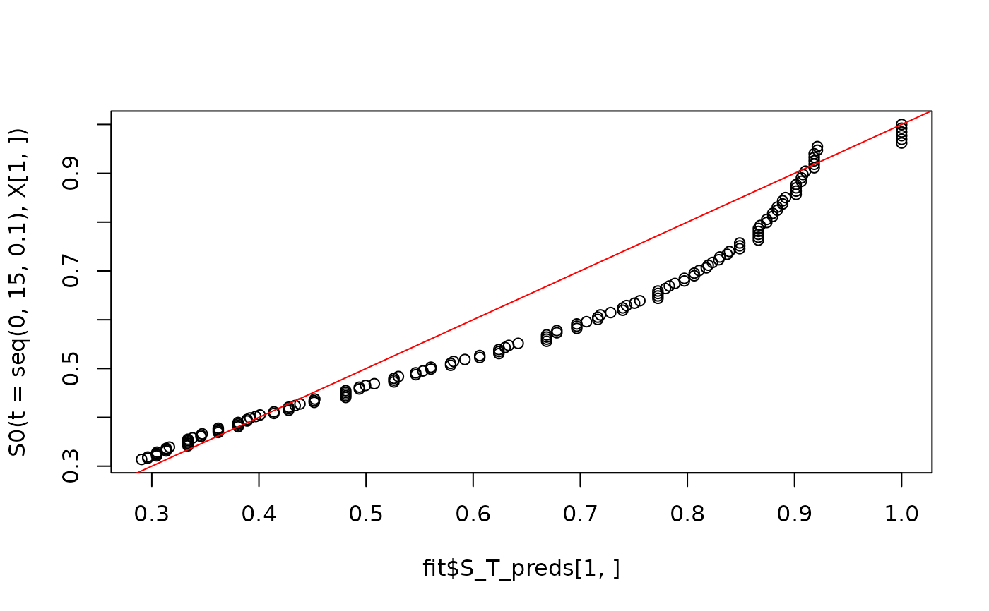
plot(fit$S_T_preds[1,], S0(t =  seq(0, 15, .1), X[1,]))
abline(0,1,col='red')