Obtain predicted conditional survival and cumulative hazard functions from a global survival stacking object
Source:R/stackG.R
predict.stackG.RdObtain predicted conditional survival and cumulative hazard functions from a global survival stacking object
Usage
# S3 method for class 'stackG'
predict(
  object,
  newX,
  newtimes,
  surv_form = object$surv_form,
  time_grid_approx = object$time_grid_approx,
  ...
)
Arguments
- object
Object of class
stackG- newX
m x pdata.frame of new observed covariate values at which to obtainmpredictions for the estimated algorithm. Must have the same names and structure asX.- newtimes
k x 1numeric vector of times at which to obtainkpredicted conditional survivals.- surv_form
Mapping from hazard estimate to survival estimate. Can be either
"PI"(product integral mapping) or"exp"(exponentiated cumulative hazard estimate). Defaults to the value saved inobject.- time_grid_approx
Numeric vector of times at which to approximate product integral or cumulative hazard interval. Defaults to the value saved in
object.- ...
Further arguments passed to or from other methods.
Value
A named list with the following components:
- S_T_preds
An
m x kmatrix of estimated event time survival probabilities at themcovariate vector values andktimes provided by the user innewXandnewtimes, respectively.- S_C_preds
An
m x kmatrix of estimated censoring time survival probabilities at themcovariate vector values andktimes provided by the user innewXandnewtimes, respectively.- Lambda_T_preds
An
m x kmatrix of estimated event time cumulative hazard function values at themcovariate vector values andktimes provided by the user innewXandnewtimes, respectively.- Lambda_C_preds
An
m x kmatrix of estimated censoring time cumulative hazard function values at themcovariate vector values andktimes provided by the user innewXandnewtimes, respectively.- time_grid_approx
The approximation grid for the product integral or cumulative hazard integral, (user-specified).
- surv_form
Exponential or product-integral form (user-specified).
Examples
# This is a small simulation example
set.seed(123)
n <- 250
X <- data.frame(X1 = rnorm(n), X2 = rbinom(n, size = 1, prob = 0.5))

S0 <- function(t, x){
  pexp(t, rate = exp(-2 + x[,1] - x[,2] + .5 * x[,1] * x[,2]), lower.tail = FALSE)
}
T <- rexp(n, rate = exp(-2 + X[,1] - X[,2] + .5 *  X[,1] * X[,2]))

G0 <- function(t, x) {
  as.numeric(t < 15) *.9*pexp(t,
                              rate = exp(-2 -.5*x[,1]-.25*x[,2]+.5*x[,1]*x[,2]),
                              lower.tail=FALSE)
}
C <- rexp(n, exp(-2 -.5 * X[,1] - .25 * X[,2] + .5 * X[,1] * X[,2]))
C[C > 15] <- 15

entry <- runif(n, 0, 15)

time <- pmin(T, C)
event <- as.numeric(T <= C)

sampled <- which(time >= entry)
X <- X[sampled,]
time <- time[sampled]
event <- event[sampled]
entry <- entry[sampled]

# Note that this a very small Super Learner library, for computational purposes.
SL.library <- c("SL.mean", "SL.glm")

fit <- stackG(time = time,
              event = event,
              entry = entry,
              X = X,
              newX = X,
              newtimes = seq(0, 15, .1),
              direction = "prospective",
              bin_size = 0.1,
              time_basis = "continuous",
              time_grid_approx = sort(unique(time)),
              surv_form = "exp",
              learner = "SuperLearner",
              SL_control = list(SL.library = SL.library,
                                V = 5))

preds <- predict(object = fit,
                 newX = X,
                 newtimes = seq(0, 15, 0.1))

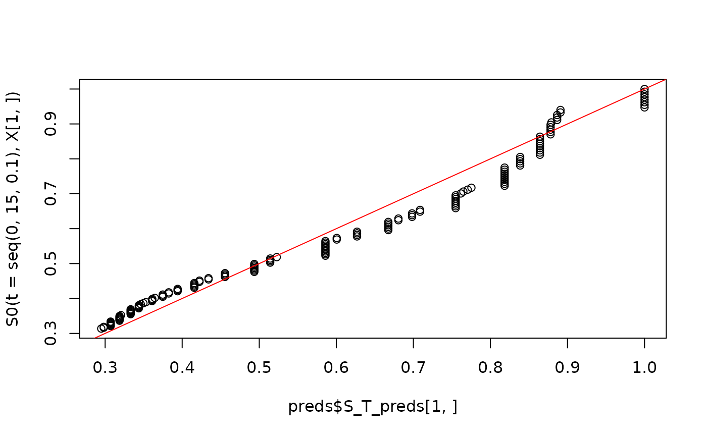
plot(preds$S_T_preds[1,], S0(t =  seq(0, 15, .1), X[1,]))
abline(0,1,col='red')
